¶ Technology Roadmap Sections and Deliverables
Unique identifier:
- 3RF-Random Forest
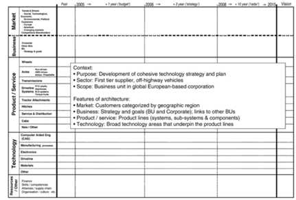
This is a “level 3” roadmap at the technology/capability level (see Fig. 8-5 of Chapter 8), where “level 1” would indicate a market level roadmap and “level 2” would indicate a product/service level technology roadmap:
Machine learning - the type of data analysis that automates analytical model building - is a vast topic that includes many different methods. Random Forest is one such method. In order to scope our group's project, we chose Random Forest as the technology of focus for our roadmap.
¶ Roadmap Overview
The basic high-level structure of Random Forest machine learning algorithms is depicted in the figure below:
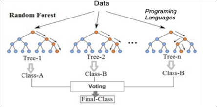
Random Forest is a classification method/technique that is based on decision trees. Classification problems are a big part of machine learning because it is important to know what classification/group observations are in. There are many classification algorithms used in data analysis such as logistic regression, support vector machine, Bayes classifier, and decision trees. Random forest is near the top of the classifier hierarchy.
Unlike the traditional decision tree classification technique, a random forest classifier grows many decision trees in ways that can address the model. In the traditional decision tree classification, there is an optimal split, which is used to decide if a property is to be true/false. Random forest contains several such trees as a forest that operate as an ensemble and allows users to make several binary splits in the data and establish complex rules for classification. Each tree in the random forest outputs a class prediction and the class with the most votes becomes the model’s prediction. Majority wins. A large population of relatively uncorrelated models operating as a committee will outperform individual constituent models. For a random forest to perform well: (1) there needs to be a signal in the features used to build the random forest model that will show if the model does better than random guessing, and (2) the prediction and errors made by the individual trees have to have low correlations with each other.
Two methods can be used to ensure that each individual tree is not too correlated with the behavior of any other trees in the model:
- Bagging (Bootstrap Aggregation) - Each individual tree randomly samples from the dataset with replacement, resulting in different trees.
- Feature Randomness - Instead of every tree being able to consider every possible feature and pick the one that produces the most separation between the observations in the left and right node, the trees in the random forest can only pick from a random subset of features. This forces more variation amongst the trees in the model, which results in lower correlation across trees and more diversification.
Trees are not only trained on different sets of data, but they also use different features to make decisions.
The random forest machine learning algorithm is a disruptive technological innovation (a technology that significantly shifts the competition to a new regime where it provides a large improvement on a different FOM than the mainstream product or service) because it is:
- versatile - can do regression or classification tasks; can handle binary, categorical, and numerical features. Data requires little pre-processing (no rescaling or transforming)
- parallelizable - process can be split to multiple machines, which results in significantly faster computation time
- effective for high dimensional data - algorithm breaks down large datasets into smaller subsets
- fast - each tree only uses a subset of features, so the model can use hundreds of features. It is quick to train
- robust - bins outliers and is indifferent to non-linear features
- low bias, moderate variance - each decision tree has a high variance but low bias; all the trees are averaged, so model how low bias and moderate variance
As a result, compared with the traditional way of having one operational model, random forest has extraordinary performance advantages based on the FOMs such as accuracy and efficiency because of the large number of models it can generate in a relatively short period of time. One interesting case of random forest increasing accuracy and efficiency is in the field of investment. In the past, investment decisions relied on specific models built by analysts. Inevitably, there were loose corners due to the reliance on single models. Nowadays, random forest (or machine learning at a larger scale) enables many models to be generated quickly to ensure the creation of a more robust decision-making solution that builds a “forest” of highly diverse "trees". This has significantly changed the industry in terms of efficiency and accuracy. For example, in a research paper by Luckyson Khaidem, et al (2016), the ROC curve shows great accuracy by modeling Apple's stock performance, using random forest. The paper also showed the continuous improvement of accuracy when applying machine learning. As a result, random forest/machine learning has significantly changed the way the investment sector operates.
¶ Design Structure Matrix (DSM) Allocation

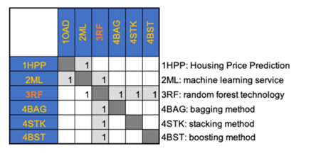
The 3-RF tree that we can extract from the DSM above shows us that the Random Forest(3RF) is part of a larger data analysis service initiative on Machine Learning (ML), and Machine Learning is also part of a major marketing initiative (here we use housing price prediction in real estate industry as an example). Random forest requires the following key enabling technologies at the subsystem level: Bagging (4BAG), Stacking (4STK), and Boosting (4BST). These three are the most common approaches in random forest, and are the technologies and resources at level 4.
¶ Roadmap Model using OPM
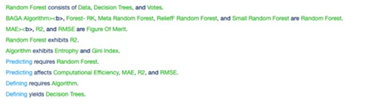
We provide an Object-Process-Diagram (OPD) of the 3RF roadmap in the figure below. This diagram captures the main object of the roadmap (random forest), its various instances with a variety of focus, its decomposition into subsystems (data, decision trees, votes), its characterization by Figures of Merit (FOMs) as well as the main processes (defining, predicting).
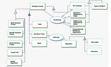
An Object-Process-Language (OPL) description of the roadmap scope is auto-generated and given below. It reflects the same content as the previous figure, but in a formal natural language.
¶ Figures of Merit (FOM)
The table below shows a list of Figures of Merit (FOM) by which the random forest models can be assessed:
Figure 5. Table of Random Forest FOM – File missing when checked in Oct 2025
The first three are used to assess the accuracy of the model:
- R-squared (R^2): a statistical measure that represents the proportion of the variance for a dependent variable that's explained by an independent variable or variables in a regression model. It is calculated by dividing the sum of squared residuals (SSR) - the sum over all observations of the squares of deviations (the difference between observed values and the values estimated by the model) - by the total sum of squares (SST) - the sum over all observations of the squared differences of each observed value from the overall mean of observed values.
Here are the variables used in the R^2 equation, explained (Variables are written in LaTeX format):
- y_i - observed value
- \hat y - value estimated by the model
- \bar y - overall mean of observed values
- Mean Absolute Error (MAE): the average magnitude of the errors in a set of predictions, without considering their direction. It’s the average over the test sample of the absolute differences between values predicted by the model and observed values where all individual differences have equal weight.
Here are the variables used in the R^2 equation, explained (Variables are written in LaTeX format):
- y_{(pred),i} - value predicted by the model
- y_i - observed value
- n - number of observations
- Root Mean Squared Error (RMSE): a quadratic scoring rule that also measures the average magnitude of the error. It’s the square root of the average of squared differences between predicted and observed values. Compared to MAE, RMSE gives a relatively high weight to large errors. This means the RMSE should be more useful when large errors are particularly undesirable.
Here are the variables used in the R^2 equation, explained (Variables are written in LaTeX format):
- \hat y_i - value predicted by the model
- y_i - observed value
- n - number of observations
Among all three, the RMSE is a FOM commonly used to measure the performance of predictive models. Since the errors are squared before they are averaged, the RMSE gives a relatively high weight to larger errors in comparison to other performance measures such as R^2 and MAE. To measure prediction, the RMSE should be calculated with out-of-sample data that was not used for model training. From a mathematical standpoint, RMSE can vary between positive infinity and zero. A very high RMSE indicates that the model is very poor at out-of-sample predictions. While an RMSE of zero is theoretically possible, this would indicate perfect prediction and is extremely unlikely in real-world situations.
Computational Efficiency is a property of an algorithm/model which relates to the number of computational resources used by the algorithm. Algorithms must be analyzed to determine resource usage, and the efficiency of an algorithm can be measured based on the usage of different resources (eg. time, space, energy, etc). Higher efficiency is achieved by minimizing resource usage. Different resources such as time and space complexity cannot be compared directly, so determining which algorithms are "more efficient" often depends on which measure of efficiency is considered most important.
Interpretability is a subjective metric used to evaluate how the analytical model works and how the results were produced. Since computers do not explain the results of the algorithms they run, and especially since model building is automated in machine learning, explaining machine learning models is a big problem that data scientists face because these machine learning models behave similarly to a "black box". The automated nature of these algorithms makes it hard for humans to know exactly what processes computers are performing. High interpretability means that the model is relatively explainable, which usually results from higher human involvement in the development and testing of the model. Models with lower interpretability are harder to rely on since the automated internal processes used to develop the model are not be clear to human users who may be less confident in the accuracy of the results.
Simplicity is a metric used to evaluate how simple/complex a model is. Simplicity is measured by taking the reciprocal of the product of the number of variables and the number of models. Complex problems do not always require complex solutions, and simple regressions are able to produce accurate results to some extent. However, there is certainly a tradeoff between simplicity and accuracy. A model could be very simple but not be able to capture the nuances of the data. On the other hand, a model could be very complex and have many variables that help to represent the data but suffer in terms of efficiency
Due to the nature of this technology, it's been challenging to quantify the growth of FOM over time, because it's not only related to the technology itself (algorithms), but also the dataset, as well as parameters selected for modeling, such as the number of trees, etc. We've tried to use the same dataset to run three models with optimized parameters, and the chart below shows the difference in RMSE metrics of the three models (Linear Regression, CART, and Random forest) compared to the years the model types were first developed.
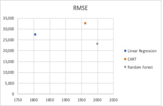
Random forest, the most recent of all three model types being compared, has the lowest RMSE value, which shows that the average magnitude of the model's error is the lowest of all three models.
Random forest is still being rapidly developed with tremendous efforts from research institutions around the world. There are also many efforts to implement and apply random forest algorithms to major industries such as: finance, investment, service, tech, energy, etc.
¶ Alignment with Company Strategic Drivers
In this section and following sections, we've embedded data analytics in real estate industry. Assuming we have a company in which we use random forest to predict housing price (like what Zillow etc. does). A dataset is used to the quantification discussion, which includes
- 2821 observations (houses' information)
- 73 independent variables, such as lot area, garage size, etc.
- 1 dependent variable: sale price
The table below shows the strategic drivers of our hypothetical company and alignment of the 3RF technology roadmap with it.
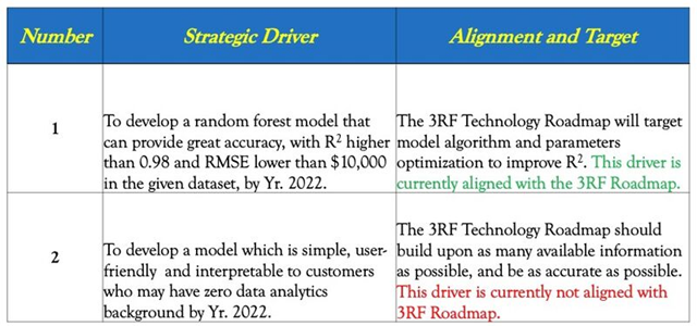
The first strategic driver indicates the company aims to improve the accuracy of the model, whereas the 3RF roadmap is also optimizing the algorithm and parameters to fine tune the model. As a result, this driver is aligned with 3RF roadmap. The second driver indicates the company is looking for simplicity, and this is not aligned with the current 3RF roadmap. This discrepancy needs immediate attention and be worked to address.
¶ Positioning of Company vs. Competition
The figure below shows a summary of other real estate companies who also use data analytics to predict housing price.
Error creating thumbnail: File missing when checked in Oct 2025
Figure 8. Competitors at Marketplace
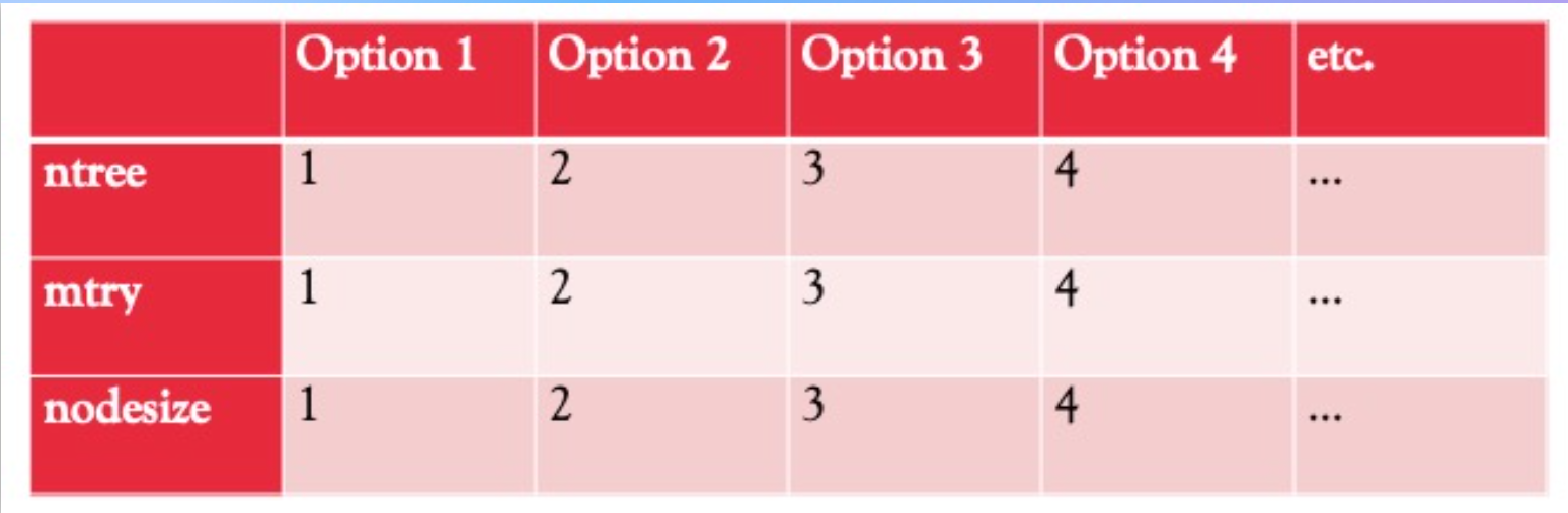
The table below shows a comparison between different companies, including the models' set up.
- ntree: number of trees (models) in the forest
- mtry: number of variables examined at each split of the trees
- nodesize: minimum number of observations in each terminal node of the trees
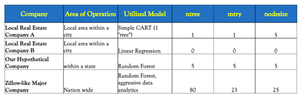
Zillow-like major company tend to have very high R2, which heavily utilize data analytics in their price prediction model. To have great accuracy, it would include as many variables information as possible, as many observations as possible. This will help to "train" their model to be very smart. Meanwhile, they have sacrificed simplicity with the many variables, and a large number of models built for machine learning purposes. Whereas some local "mom and pop stores" would utilize very simple models such as linear regression or CART, of which the accuracy of the model is sacrificed. Right now our hypothetical company is trying to utilize random forest to deliver good accuracy while still maintain a certain level of simplicity
(In this chart, the simplicity is defined as reciprocal of the number of variables and number of models. For example, our hypothetical company uses 73 variables and 5 models for prediction, the simplicity is 1/(73*5)=0.0027. The more variables or more models our prediction relies on, the lower the simplicity. This is aligned with our intuition)
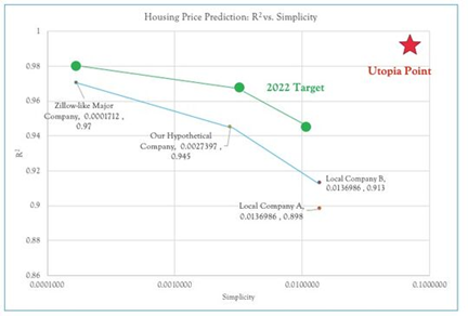
The Pareto Front (for this specific dataset) is shown in blue line. It's clear that the local company A (using CART)is not at the Pareto Front, instead, it would be dominated. The local company B using linear regression is as simple, but the accuracy is better. Zillow-like major company and our hypothetical company both are much better in terms of accuracy.
For the target of Yr. 2020, the green line defines the expected Pareto Front at then. Comparing with current performance, the future Pareto Front is expected to improve either accuracy (R2), or simplicity, or both. The company's strategy will determine the direction, and extent of improvement.
¶ Technical Model
An example morphological matrix is developed for 3RF roadmap in this specific case. The purpose of such a model is to understand all the design vectors, explore the design tradespace and establish what are the active constraints in the system.
Due to the special nature of this technology, there is no defined equations for the FOM’s. The FOM’s values are impacted by the model parameters, including ntree, nodsize, mtry (w/o clearly defined mathematical equations or regression equations), and the dataset, including all variables and observations.
Explanation of parameters:
1) ntree: number of CART trees in the forest
2) mtry: number of variables examined at each split of the trees
3) nodesize: minimum number of observations in each terminal node of the trees
As a result, for any given dataset, the expressions of two FOM’s can be expressed in this way:
R2 ∼ f1 (ntree, nodesize, mtry)
RMSE ∼ f2 (ntree, nodesize, mtry)
One dataset is used to normalize any potential difference caused by data source. This dataset is from the real estate industry with 2821 observations (houses' information),73 independent variables, such as lot area, garage size, etc., and 1 dependent variable (sale price). The goal of the model is to predict sale price based on these 73 independent variables.
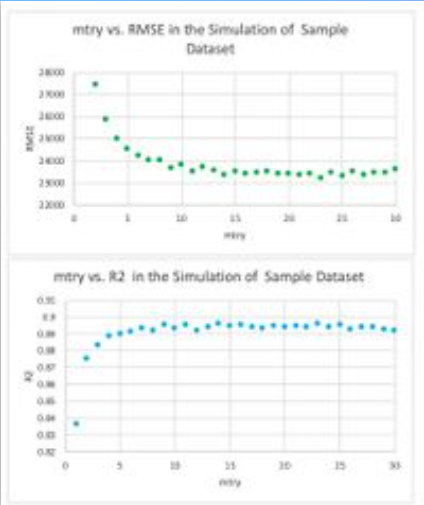
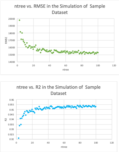
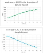
Notional trends: each dot on the plot represent the output of the corresponding FOM (R2 or RMSE) at the given value of the parameter while fixing other parameters
These two charts below show the impact of mtry on the 2 FOMs:
These two charts below show the impact of ntree on the 2 FOMs:
These two charts below show the impact of node size on the 2 FOMS's:

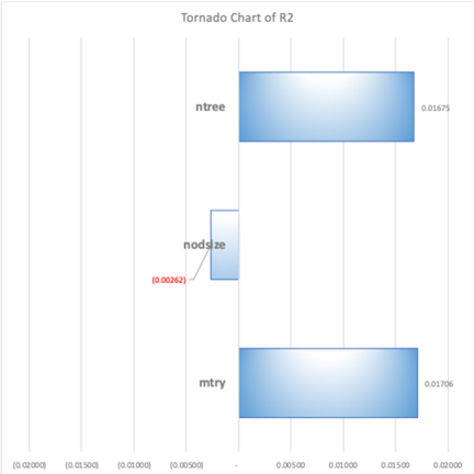
Because there is no governing equation, no partial derivative can be drawn to illustrate the difference. From previous notional trends, it’s also clear the finite difference also changes, even the direction of the difference (positive or negative). As a result, a baseline model with a set of inputs was defined; by verifying the values of the inputs in different models, tornado charts were generated to represent the finite difference of baseline caused by these changes. With all the given conditions, both ntree and mtry are very critical to the performance; both FOM’s are mostly sensitive to mtry
Error creating thumbnail: File missing when checked in Oct 2025
Figure 16. Tornado Chart of RMSE
Based on the preliminary results on sensitivity, and background knowledge on Random forest, the R&D focus should be on mtry optimization, because 1) it's very sensitive, and plays a big difference in the result of the model- lower or higher than the optimal value will both deteriorate the result; 2) in random forest, mtry is a key factor to determine two critical aspects: diversity of the models which tend to favor a smaller mtry, and performance of the models which tend to favor a larger mtry. Accordingly, optimizing mtry is critical. Meanwhile, it's also worth to point out that the mtry optimization need to rely on ntree and nodesize as well. As a result, the approach should be to find the optimal algorithm to optimize all three parameters but focusing on mtry.
¶ Financial Model
The figure below contains a sample NPV analysis underlying the 3RF roadmap. It shows the initial non-recurring cost of the project development for the first 2 years for the research projects, before revenue starts generating since Yr. 3. The ramp up period is around 6 years, until the market is situated with revenue of around $8MM/year. Total estimated project life is 17 years.
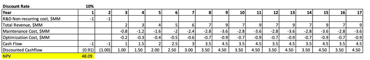
Based on our outlook, the revenue will be stabilized around $8MM, however, there is significant uncertainty on market demand as well as the organization capability to keep up with the technology development year by year. As a result, we introduced an oscillation factor so the revenue will be bouncing between $7MM and $9MM. The underlying assumption is if the revenue is lower than $8MM in one year, more efforts will be in place the next year to improve the revenue to be $9MM. Meanwhile, the maintenance and operations cost will oscillate with revenue, because more efforts on improving revenue will likely require higher operations and maintenance cost.
Error creating thumbnail: File missing when checked in Oct 2025
Figure 17.2 Cash Flow Representation
¶ List of R&T Projects and Prototypes
To plan and prioritize R&D or R&T projects, we use the strategic drivers of the company as overarching principles and technical models and financial models as guiding principles to develop the project categories and roadmaps.
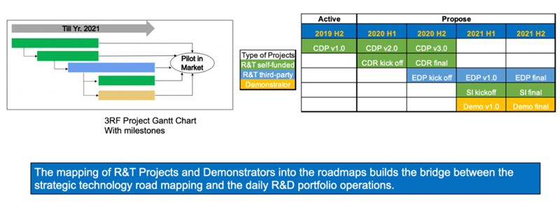
Five Projects will be the focus in near future:
- Current database model performance optimization (CDP)
- Current database robustness optimization (CDR)
- Expanded database performance and robustness optimization (EDP)
- Simplicity and interpretability optimization (SI)
- Demonstrator (Demo)
Project Gantt chart is developed to represent the sequence and resource requirements for different projects. The projects were also paced out to be aligned with R&D budget outlook of each year:
¶ Key Publications, Presentations and Patents
Part 1: Key Patents for Random Forest
- U.S. Patent 6009199 by Tin Kam Ho from Bell Lab: Introduction of random forest- a decision forest including multiple decision trees is used to classify "seen" training data and "unseen" data. Each individual tree performs an initial classification based on randomly selected subsets of the data. The classification outcomes by the individual trees are combined using a discriminant process in the decision-forest classier to render the ultimate classification decision. https://patents.google.com/patent/US6009199A/en
Part 2: Publications on the Development of Random Forest:
- The very first paper on random forest, published by Tin Kam Ho from Bell Laboratories. It introduced the method to construct tree-based classifiers whose capacity can be arbitrarily expanded for increased in accuracy for both training and unseen data, by following the principles of stochastic modeling. https://web.archive.org/web/20160417030218/http://ect.bell-labs.com/who/tkh/publications/papers/odt.pdf
- This is an early paper published by Yali Amit and Donald Geman on shaping quantization and recognition with randomized trees. This will be a good reading to understand the early development and application of random forest. http://www.cis.jhu.edu/publications/papers_in_database/GEMAN/shape.pdf
- This is a paper published by Tin Kam Ho on the optimization of random forest. It introduced a method to construct a decision tree based classifier is proposed that maintains the highest accuracy on training data and improves on generalization accuracy as it grows in complexity. The classifier consists of multiple trees constructed systematically by pseudorandomly selecting subsets of components of the feature vector, that is, trees constructed in randomly chosen subspaces. The subspace method is compared to single-tree classifiers and other forest construction methods by experiments on publicly available datasets, where the method's superiority is demonstrated. https://ieeexplore.ieee.org/document/709601
- This is a research paper published by Thomas Dietterich on a comparison of three methods for constructing random forest: bagging, boosting, and randomization. Bagging and boosting are methods that generate a diverse ensemble of classifiers by manipulating the training data given to a “base” learning algorithm. An alternative approach to generating an ensemble is to randomize the internal decisions made by the base algorithm. This paper compares the effectiveness of randomization, bagging, and boosting for improving the performance of the decision-tree algorithm C4.5. The experiments show that in situations with little or no classification noise, randomization is competitive with (and perhaps slightly superior to) bagging but not as accurate as boosting. In situations with substantial classification noise, bagging is much better than boosting, and sometimes better than randomization. https://link.springer.com/content/pdf/10.1023/A:1007607513941.pdf
- This is a very impactful paper published by Leo Breiman in UC Berkeley: The generalization error of a forest of tree classifiers depends on the strength of the individual trees in the forest and the correlation between them. Using a random selection of features to split each node yields error rates that compare favorably to Adaboost (Freund and Schapire[1996]), but are more robust with respect to noise. Internal estimates monitor error, strength, and correlation and these are used to show the response to increasing the number of features used in the splitting. Internal estimates are also used to measure variable importance. These ideas are also applicable to regression. https://www.stat.berkeley.edu/~breiman/randomforest2001.pdf
Part 3: Key References on Data Analytics in Real Estate Industry:
- This paper is published by An Nguyen in Yr. 2018 regarding housing price prediction. This paper explores the question of how house prices in five different counties are affected by housing characteristics (both internally, such as number of bathrooms, bedrooms, etc. and externally, such as public schools’ scores or the walkability score of the neighborhood). This paper utilizes both the hedonic pricing model (Linear Regression) and various machine learning algorithms, such as Random Forest (RF) to predict house prices. https://pdfs.semanticscholar.org/782d/3fdf15f5ff99d5fb6acafb61ed8e1c60fab8.pdf
- This is a great introduction on how data analytics can be used to predict housing prices. Examples include using heat maps to show correlations among features and sale price and using random forest to build a model for prediction purposes. https://towardsdatascience.com/home-value-prediction-2de1c293853c
- This is a great explanation of how random forest analysis is used in predicting housing prices. It includes the interpretation of random forests, parameter tuning of random forest, and feature importance based on the results. https://medium.com/@santhoshetty/predicting-housing-prices-4969f6b0945
- This is a great reading on the utilization of multiple models to predict housing prices, from linear regression, log regression, to random forest, SVM, etc. It also includes the optimization of different models. http://terpconnect.umd.edu/~lzhong/INST737/milestone2_presentation.pdf
- This reading is all about predicting house prices using machine learning algorithms. It utilized a dataset from Kaggle, and then step-by-step analyzed the data, with great visualization and quantitative output. https://nycdatascience.com/blog/student-works/housing-price-prediction-using-advanced-regression-analysis/
Part 4: Extended Reading- Interesting Random Forest applications in many other fields:
- Using Random Forests on Real-World City Data for Urban Planning in a Visual Semantic Decision Support System: A preeminent problem affecting urban planning is the appropriate choice of location to host a particular activity (either commercial or common welfare service) or the correct use of an existing building or empty space. The proposed system in this research paper combines, fuses, and merges various types of data from different sources, encodes them using a novel semantic model that can capture and utilize both low-level geometric information and higher-level semantic information and subsequently feeds them to the random forests classifier, as well as other supervised machine learning models for comparisons. https://www.ncbi.nlm.nih.gov/pmc/articles/PMC6567884/
- Random Forest ensembles for detection and prediction of Alzheimer's disease with good between-cohort robustness: Computer-aided diagnosis of Alzheimer's disease (AD) is a rapidly developing field of neuroimaging with strong potential to be used in practice. In this context, assessment of models' robustness to noise and imaging protocol differences together with post-processing and tuning strategies are key tasks to be addressed in order to move towards successful clinical applications. In this study, we investigated the efficacy of Random Forest classifiers trained using different structural MRI measures, with and without neuroanatomical constraints in the detection and prediction of AD in terms of accuracy and between-cohort robustness. https://www.sciencedirect.com/science/article/pii/S2213158214001326
- A Random Forest approach to predict the spatial distribution of sediment pollution in an estuarine system: Modeling the magnitude and distribution of sediment-bound pollutants in estuaries is often limited by incomplete knowledge of the site and inadequate sample density. To address these modeling limitations, a decision-support tool framework was conceived that predicts sediment contamination from the sub-estuary to broader estuary extent. For this study, a Random Forest (RF) model was implemented to predict the distribution of a model contaminant. https://journals.plos.org/plosone/article?id=10.1371/journal.pone.0179473
- Towards Automatic Personality Prediction Using Facebook Like Categories: Effortlessly accessible digital records of behavior such as Facebook Likes can be obtained and utilized to automatically distinguish a wide range of highly delicate personal traits, including: life satisfaction, cultural ethnicity, political views, age, gender and personality traits. The analysis presented based on a dataset of over 738,000 users who conferred their Facebook Likes, social network activities, egocentric network, demographic characteristics, and the results of various psychometric tests for our extended personality analysis. The proposed model uses unique mapping technique between each Facebook Like object to the corresponding Facebook page category/sub-category object, which is then evaluated as features for a set of machine learning algorithms to predict individual psycho-demographic profiles from Likes. The model properly distinguishes between a religious and nonreligious individual in 83% of circumstances, Asian and European in 87% of situations, and between emotional stable and emotion unstable in 81% of situations. https://arxiv.org/ftp/arxiv/papers/1812/1812.04346.pdf
- CPEM: Accurate cancer type classification based on somatic alterations using an ensemble of a random forest and a deep neural network: With recent advances in DNA sequencing technologies, fast acquisition of large-scale genomic data has become commonplace. For cancer studies, in particular, there is an increasing need for the classification of cancer type based on somatic alterations detected from sequencing analyses. However, the ever-increasing size and complexity of the data make the classification task extremely challenging. In this study, we evaluate the contributions of various input features, such as mutation profiles, mutation rates, mutation spectra and signatures, and somatic copy number alterations that can be derived from genomic data, and further utilize them for accurate cancer type classification. We introduce a novel ensemble of machine learning classifiers, called CPEM (Cancer Predictor using an Ensemble Model), which is tested on 7,002 samples representing over 31 different cancer types collected from The Cancer Genome Atlas (TCGA) database. We first systematically examined the impact of the input features. Features known to be associated with specific cancers had relatively high importance in our initial prediction model. We further investigated various machine learning classifiers and feature selection methods to derive the ensemble-based cancer type prediction model achieving up to 84% classification accuracy in the nested 10-fold cross-validation. Finally, we narrowed down the target cancers to the six most common types and achieved up to 94% accuracy. https://www.nature.com/articles/s41598-019-53034-3
- Facebook Engineering: Under the hood - Suicide prevention tools powered by AI: Suicide is the second most common cause of death for people ages 15-29. Research has found that one of the best ways to prevent suicide is for those in distress to hear from people who care about them. Facebook is well positioned — through friendships on the site — to help connect a person in distress with people who can support them. It’s part of our ongoing effort to help build a safe community on and off Facebook. We recently announced an expansion of our existing suicide prevention tools that use artificial intelligence to identify posts with language expressing suicidal thoughts. We’d like to share more details about this, as we know that there is growing interest in Facebook’s use of AI and in the nuances associated with working in such a sensitive space. https://engineering.fb.com/ml-applications/under-the-hood-suicide-prevention-tools-powered-by-ai/
¶ Technology Strategy Statement
Our target is to develop a real estate digital platform with integration between traditional real estate industry and state of the art data analytics. To achieve the target of an accurate prediction method for the optimal price of housing for broader customers, we will invest in two R&D categories. The first is an algorithm optimization project to improve the accuracy of current machine learning to an R^2 of 0.98 using the sample data. The second project is a user interface improvement project to make our methodology simpler to use in order to attract users. These R&D projects will enable us to reach our goal in Yr. 2022.
Error creating thumbnail: File missing when checked in Oct 2025
Figure 19. Arrow Chart for Model Development