Difference between revisions of "Sustainable Syngas"
| Line 142: | Line 142: | ||
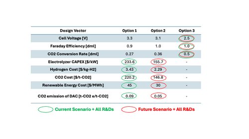
There are multiple variables in the technical models of cost and carbon intensity, described by the eqs. (7.5-9) and eq. (7.12) respectively. For an initial investigation of a tradespace, the morphological matrix is defined as shown in Table 7.1. The values of variables are determined from the reference [7.1], where the Option 1, the Option 2, and the Option 3 assumes the conservative case, the nominal case, and the optimistic case respectively. | There are multiple variables in the technical models of cost and carbon intensity, described by the eqs. (7.5-9) and eq. (7.12) respectively. For an initial investigation of a tradespace, the morphological matrix is defined as shown in Table 7.1. The values of variables are determined from the reference [7.1], where the Option 1, the Option 2, and the Option 3 assumes the conservative case, the nominal case, and the optimistic case respectively. | ||
[[File:FY24Team4_Table7.1.png|500px|thumb|center|Table 7.1: Morphological matrix]] | |||
Table 7.1: Morphological matrix | |||
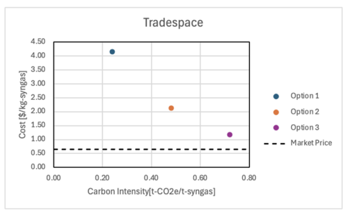
Using the values in the Table 7.1, the cost and CI are calculated and plotted in Figure 7.1. It was found that even the optimistic scenario does not meet the current market price of the syngas, which implies further technology development is required. | Using the values in the Table 7.1, the cost and CI are calculated and plotted in Figure 7.1. It was found that even the optimistic scenario does not meet the current market price of the syngas, which implies further technology development is required. | ||
Figure 7.1: Initial Tradespace | [[File:FY24Team4_Figure7.1.png|500px|thumb|center|Figure 7.1: Initial Tradespace]] | ||
<strong> Sensitivity Analysis </strong> | <strong> Sensitivity Analysis </strong> | ||
| Line 153: | Line 152: | ||
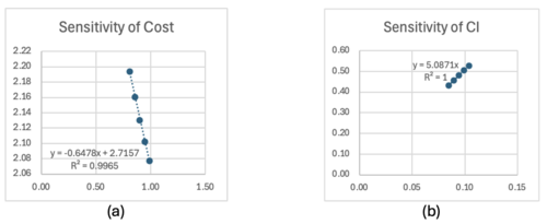
Using the technical models developed in this section, the sensitivity analysis was performed. The finite difference approach was used to estimate the sensitive of each variable. The Option 2 in Table 7.1 was used as the baseline of variables, and the variables are changed by -10%, -5%, +5%, +10%. The FOMs, i.e., cost and CI, were accordingly calculated, and the slope of FOM (dFOM/dx, where x is variable) was calculated. Figure 7.2 shows the example of dFOM/dx. All of the variables are in linear relation with the FOM, where the R2 values were close to 1. | Using the technical models developed in this section, the sensitivity analysis was performed. The finite difference approach was used to estimate the sensitive of each variable. The Option 2 in Table 7.1 was used as the baseline of variables, and the variables are changed by -10%, -5%, +5%, +10%. The FOMs, i.e., cost and CI, were accordingly calculated, and the slope of FOM (dFOM/dx, where x is variable) was calculated. Figure 7.2 shows the example of dFOM/dx. All of the variables are in linear relation with the FOM, where the R2 values were close to 1. | ||
[[File:FY24Team4_Figure7.2.png|500px|thumb|center|Figure 7.2: (a) The sensitivity of the Faraday Efficiency to the cost, and (b) the sensitivity of the CO2 emission of DAC to the carbon intensity.]] | |||
Figure 7.2: (a) The sensitivity of the Faraday Efficiency to the cost, and (b) the sensitivity of the CO2 emission of DAC to the carbon intensity. | |||
<strong> Normalized Sensitivities </strong> | <strong> Normalized Sensitivities </strong> | ||
| Line 160: | Line 158: | ||
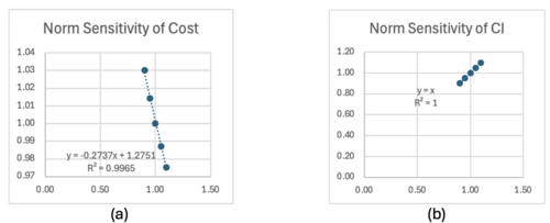
Normalized sensitivities are similarly calculated. The same approach was used as the sensitivity analysis, however, the normalized FOMS and variables were used for the finite difference calculation. Figure 7.3 shows the example of normalized dFOM/dx. All of the normalized variables are in linear relation with the normalized FOM, where the R2 values were close to 1. | Normalized sensitivities are similarly calculated. The same approach was used as the sensitivity analysis, however, the normalized FOMS and variables were used for the finite difference calculation. Figure 7.3 shows the example of normalized dFOM/dx. All of the normalized variables are in linear relation with the normalized FOM, where the R2 values were close to 1. | ||
[[File:FY24Team4_Figure7.3.png|500px|thumb|center|Figure 7.3: The normalized sensitivity of the Faraday Efficiency to the cost, and (b) the normalized sensitivity of the CO2 emission of DAC to the carbon intensity.]] | |||
Figure 7.3: The normalized sensitivity of the Faraday Efficiency to the cost, and (b) the normalized sensitivity of the CO2 emission of DAC to the carbon intensity. | |||
<strong> Tornado chart </strong> | <strong> Tornado chart </strong> | ||
| Line 168: | Line 165: | ||
On the other hand, two variables in CI model have the same sensitivity to the CI. The carbon emission in CO2 electrolysis is associated with the emission of thermal energy used in DAC. Therefore, decreasing the unreacted CO2 by increasing the CO2 conversion rate, or decreasing CO2 emission of DAC are both effective to decrease the carbon intensity. | On the other hand, two variables in CI model have the same sensitivity to the CI. The carbon emission in CO2 electrolysis is associated with the emission of thermal energy used in DAC. Therefore, decreasing the unreacted CO2 by increasing the CO2 conversion rate, or decreasing CO2 emission of DAC are both effective to decrease the carbon intensity. | ||
[[File:FY24Team4_Table7.2.png|500px|thumb|center|Table 7.2: Sensitivity and normalized sensitivity.]] | |||
[[File:FY24Team4_Figure7.4a.png|500px|thumb|center]][[File:FY24Team4_Figure7.4b.png|500px|thumb|center]] | |||
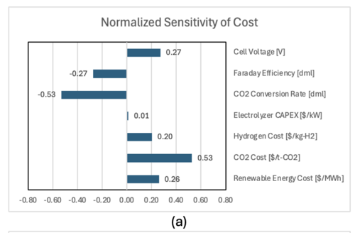
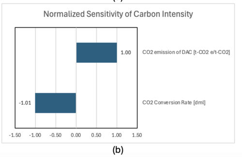
Figure 7.4: Tornado charts of the normalized sensitivity of (a) the cost and (b) the carbon intensity. | Figure 7.4: Tornado charts of the normalized sensitivity of (a) the cost and (b) the carbon intensity. | ||
== Keys Publications, Presentations and Patents == | == Keys Publications, Presentations and Patents == | ||
Revision as of 03:29, 3 November 2024
Roadmap Overview
Synthesis gas (Syngas)—a mixture of carbon monoxide (CO), hydrogen (H₂), and hydrocarbon compounds—plays a crucial role in the sustainable production of fuels used for transportation and the manufacturing of plastics. Over the years, various feedstocks have been explored to improve syngas production in terms of carbon intensity and energy efficiency.
This roadmap focuses on the production of syngas using the electrolysis of water powered by renewable energy sources such as wind, solar, or hydropower. Electrolysis splits water (H₂O) molecules into hydrogen (H₂) and oxygen (O₂). The hydrogen produced through this process combines with captured carbon dioxide (CO₂) to form carbon monoxide (CO), hydrogen (H₂), and hydrocarbon compounds. These reactions take place in two key stages:
1. Electrolysis Chamber: The process begins with water electrolysis, where electricity from renewable sources splits water into hydrogen and oxygen.
2. Reactor Chamber: In the reactor, the CO₂ feedstock is heated and reacts with the hydrogen from electrolysis in the presence of a catalyst. This process forms syngas (CO and H₂), which can be used for fuel production.
Carbon capture technology is an essential component of this system. CO₂ is captured from industrial emissions, the atmosphere, or other sources using carbon capture, utilization, and storage (CCUS) technologies. The captured CO₂ is then processed and used to react with hydrogen to produce syngas. To ensure sustainability, the system requires a constant and reliable supply of CO₂, which is achieved through advanced capture and transportation methods.
Reference Case The reference case for this technology is based on Power-to-X (P2X) solutions, where renewable electricity is converted into carbon-neutral fuels or chemicals. This approach has been applied in various pilot projects aiming to produce synthetic fuels and chemicals for industries such as transportation, plastics, and energy storage.
Key Features: a. Renewable Energy Integration: The electrolysis process is powered by clean energy sources (e.g., wind, solar, or hydro), minimizing the carbon footprint. b. Carbon Capture Utilization: CO₂ captured from the atmosphere or industrial processes is used to produce syngas, ensuring a closed carbon cycle. c. Catalyst Efficiency: The reactor employs catalysts that increase the reaction rate between hydrogen and CO₂, improving overall system efficiency.
Design Structure Matrix (DSM) Allocation
Level 1: Market Strategy
The market strategy focuses on clean energy transition and sustainable fuels. It sets performance targets like low carbon intensity, cost reduction, energy efficiency, and scalability. This is where the strategy aligns with market needs for clean energy, low-emission transportation fuels, and sustainable plastics production.
Level 2: Syngas Production The product of this strategy is syngas production through renewable energy-powered electrolysis and carbon capture. Syngas serves as an intermediate feedstock for sustainable fuel and plastic production.
Level 3: Key Enabling Component Technologies These are the subsystem-level technologies needed to drive syngas production efficiently and sustainably:
3RCC Renewable Carbon Capture (CO₂ Capture and Transport Technologies): Enables the trapping of CO₂ from industrial emissions or direct air capture, which is essential for syngas production. 3EEL Electrolysis Efficiency (High-Efficiency Electrolyzers): Focuses on electrolysis units that split water with minimal energy loss, leveraging renewable energy like solar and wind to power the system. 3CRX Catalytic Reactors for CO₂-H₂ Reactions: Catalytic systems designed to maximize the efficiency of the reaction between hydrogen and carbon dioxide to form syngas, ensuring high yield and minimal energy consumption. 3PCS Power Conditioning Systems: This system ensures that the renewable energy input is stable, reliable, and properly conditioned to meet the demands of the electrolysis and reactor processes, including day-night cycle energy management. 3ESS Energy Storage Systems: Involves the integration of energy storage solutions (e.g., lithium-ion batteries or regenerative fuel cells) to manage the intermittent nature of renewable energy sources, ensuring a consistent energy supply for the syngas production process.
Roadmap Model using Object Process Methodology (OPM)
Figure of Merit (FOM)
Alignment with Company Strategic Drivers
Positioning of Company vs. Competition
Technical Model
Governing Equations [7.1]
CO2 electrolysis is the electrochemical reduction of CO2 into various products. The selective reduction of CO2 into CO is the matured pathway in the low-temperature CO2 electrolysis, and the reaction follows the eq. (7.1);
where, the CO2 is reduced into CO at the cathode side and the oxygen evolution reaction is observed at the anode side.
The total current required for the CO2 electrolysis is calculated from the transferred electrons from the anode to the cathode by the eq (7.2);
where, I is the total current [A], FE_CO is the Faradaic efficiency, m ̇_CO is the production rate of CO [t-CO/hr], MW_CO is the molecular weight of CO [g/mol], z_(e^-,CO) is the number of electrons passed through [mol-e–/mol-CO], and F is the Faraday’s constant [C/mol]. Therefore, the power consumption of the CO2 electrolysis is calculated by the eq. (7.3);
where, P is the power consumption [MW], and V_cell is the applied voltage to the cell [V].
The energy consumption per ton of CO is similarly calculated by the eq. (7.4), considering the transferred electrons;
where, E is the energy consumption [MWh/t-CO], and n_(e^- ) is the number of required electrons.
Cost Model
In this roadmapping, the cost is chosen as one of the FOM. The cost of producing a ton of syngas is decomposed into the OPEX and the CAPEX as follows;
where, the cost, OPEX, and CAPEX are measured in $/t-syngas.
The OPEX is further decomposed into the feedstock cost and the electricity cost (eq. (7.6)). The feedstock cost is associated with the cost of hydrogen and CO2 used for CO2 electrolysis. Since the molecular ratio of hydrogen and CO2 in the syngas is 2:1, the feedstock cost is derived by the eq (7.7);
where, FS_(H_2 ) is the required amount of hydrogen [t-H2/t-syngas], C_(H_2 ) is the cost of hydrogen [$/t-H2], FS_(CO_2 ) is the required amount of CO2 [t-CO2/t-syngas], C_(CO_2 ) is the cost of CO2 [$/t-CO2], MW_(H_2 ) is the molecular weight of hydrogen [g/mol], and MW_(CO_2 ) is the molecular weight of CO2 [g/mol].
The electricity cost is derived from the energy consumption (eq. (7.4)) by adjusting its amount through the weight ratio;
The CAPEX is calculated from the sum of equipment cost and the amount of syngas production through the lifetime of equipment. The equipment cost is estimated as linear to the power consumption [7.1]. Therefore, the CAPEX is calculated by the eq. (7.9);
where, C_Electrolyzer is the cost of electrolyzer per power consumption [$/kW], ANP is the annual production of syngas [t-syngas/yr], L is the lifetime [yr].
Carbon Intensity Model
The other FOM chosen in this roadmapping is the carbon intensity (CI), which is defined as follows;
where, CI is the carbon intensity [kg-CO2e/kg-syngas], E_Feedstock is the CO2 emission associated with the feedstock processing [kg-CO2e], E_Embodied is the CO2 embodied into the product (in this case, syngas) [kg-CO2e], E_Operation is the CO2 emission during the operation and processing [kg-CO2e], and E_Sequestration is the CO2 abated through sequestration [kg-CO2e].
In this roadmapping, the assumption is made where the CO2 feedstock is obtained by the Direct Air Capture (DAC) and hydrogen is obtained by water electrolysis. The DAC reduces E_Feedstock since the CO2 is directly taken from the atmosphere. However, the process of DAC requires thermal energy that is produced by natural gas. According to the reference [7.1] and our estimation, it was found that the CO2 emission of DAC is about 0.094 [t-CO2e/t-CO2]. Therefore, E_Feedstock is decomposed as follows;
The CO2 electrolysis does not produce operational emissions. However, there are unreacted CO2 that might be released to the atmosphere and counted as E_Operation. The sum of the embodied CO2 and the unreacted CO2 is equal to the captured CO2 in eq. (7.11). Considering there is no CO2 sequestration, the eq. (7.10) is simplified as follows;
where, E_DAC is the carbon emission of DAC to capture a ton of CO2 [t-CO2e/t-CO2] and is equal to 0.094.
Morphological Matrix and Initial Definition of Tradespace
There are multiple variables in the technical models of cost and carbon intensity, described by the eqs. (7.5-9) and eq. (7.12) respectively. For an initial investigation of a tradespace, the morphological matrix is defined as shown in Table 7.1. The values of variables are determined from the reference [7.1], where the Option 1, the Option 2, and the Option 3 assumes the conservative case, the nominal case, and the optimistic case respectively.
Using the values in the Table 7.1, the cost and CI are calculated and plotted in Figure 7.1. It was found that even the optimistic scenario does not meet the current market price of the syngas, which implies further technology development is required.
Sensitivity Analysis
Using the technical models developed in this section, the sensitivity analysis was performed. The finite difference approach was used to estimate the sensitive of each variable. The Option 2 in Table 7.1 was used as the baseline of variables, and the variables are changed by -10%, -5%, +5%, +10%. The FOMs, i.e., cost and CI, were accordingly calculated, and the slope of FOM (dFOM/dx, where x is variable) was calculated. Figure 7.2 shows the example of dFOM/dx. All of the variables are in linear relation with the FOM, where the R2 values were close to 1.
Normalized Sensitivities
Normalized sensitivities are similarly calculated. The same approach was used as the sensitivity analysis, however, the normalized FOMS and variables were used for the finite difference calculation. Figure 7.3 shows the example of normalized dFOM/dx. All of the normalized variables are in linear relation with the normalized FOM, where the R2 values were close to 1.
Tornado chart
The results of sensitivity analysis are summarized in Table 7.2, and the tornado charts of normalized sensitivity are described in Figure 7.4. It was found that the cost and the conversion rate of CO2 are most sensitive to the syngas cost. This is because the production of syngas requires the same amount of CO2 in mole. Considering that only 27% of the CO2 is converted into CO in the baseline, there are space in CO2 conversion rate for technical development. On the other hand, two variables in CI model have the same sensitivity to the CI. The carbon emission in CO2 electrolysis is associated with the emission of thermal energy used in DAC. Therefore, decreasing the unreacted CO2 by increasing the CO2 conversion rate, or decreasing CO2 emission of DAC are both effective to decrease the carbon intensity.
Figure 7.4: Tornado charts of the normalized sensitivity of (a) the cost and (b) the carbon intensity.


